MATLAB code Bisection Method (root)

%Bisection method
%Step 1: Choose lower xl and upper xu guesses for
%the root such that the function changes sign
%over the interval. This can be checked by ensuring
%that f(xl)*f(xu) < 0.
%Step 2: An estimate of the root xr is determined
%by xr = (xl + xu)/2
%Step 3: Make the following evaluations to determine
%in which subinterval the root lies:
%(a) If f(xl)f(xr) < 0, the root lies in the lower
%subinterval. Therefore, set xu 5 xr and return to step 2.
%(b) If f(xl)f(xr) > 0, the root lies in the upper
%subinterval. Therefore, set xl 5 xr and return to step 2.
%(c) If f(xl)f(xr) = 0, the root equals xr; terminate the computation.

%Example

Parallel with R. Example with snow

Snow provides support for easily executing R functions in parallel. Most of the parallel execution functions in snow are variations of the standard lapply() function, making snow fairly easy to learn. To implement these parallel operations, snow uses a master/ worker architecture, where the master sends tasks to the workers, and the workers execute the tasks and return the results to the master.

The basic cluster creation function is makeCluster() which can create any type of cluster. snow includes a number of functions that we could use, including clusterApply(), clusterApplyLB(), and parLapply(). For this example, we’ll use clusterApply(). You call it exactly the same as lapply(), except that it takes a snow cluster object as the first argument. We also need to load MASS on the workers, rather than on the master, since it’s the workers that use the “Boston” dataset.

We’ll use snow.time() to gather timing information about the overall execution. We will also use snow.time()’s plotting capability to visualize the task execution on the workers. 

Bisection method, Java code

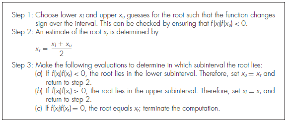
The bisection method, which is alternatively called binary chopping, interval halving, or Bolzano’s method, is one type of incremental search method in which the interval is always divided in half. If a function changes sign over an interval, the function value at the midpoint is evaluated. The location of the root is then determined as lying at the midpoint of the subinterval within which the sign change occurs. The process is repeated to obtain refined estimates. A simple algorithm for the bisection calculation is listed in the following figure.

Reference; Numerical Methods for Engineers. Steven C. Chapra and Raymond P. Canale

Lagrange Polynomial Java code

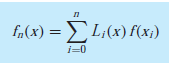
The Lagrange interpolating polynomial is simply a reformulation of the Newton polynomial
that avoids the computation of divided differences. It can be represented concisely as

where

Linear Interpolation code C# and FORTRAN

With this method any two points are simple joined together by a straight line segment. The desired interpolation point should therefore lie on this same line segment. The next codes calculate single point linear interpolation (xval,yval) using to vectors data (x,y).


You can this code to linear interpolation in FORTRAN

       

SUBROUTINE LinearInterpolation(x,y,xval,yval,n)
  real::x(n),y(n),xval,yval
  integer::n,i
     yval = 0
     do i=1,n
  
   IF (xval >= x(i) .AND. xval < x(i+1)) then   
   
   yval = y(i)+(xval-x(i))*(y(i+1)-y(i))/(x(i+1)-x(i));
 
   end if
      end do
   return
   
      end SUBROUTINE 

Reservoir simulation code (1D-horizontal-single phase) FORTRAN

With this code you can practice with examples of reservoir simulation excersices with the follows considerations:

One dimension
Horizontal
One phase (oil)
Slightly compressible fluid
4 different types of boundary conditions
Implicit formulation
Peaceman well model
One well (specified production rate or specified flowing pressure)

You can change the number of cells, rock and fluid properties, boundaries conditions and well especification.

Z-factor: Dranchuk-Purvis-Robinson correlation C# code

Code to calculate Z factor with Dranchuk-Purvis-Robinson Method in C#.

Dranchuk et. al. (1974) developed a correlation based on the Benedict-Webb-Rubin type of equation of state. Fittig the equation to 1500 data points from the Standing and Katz Z-factor chart optimized the eight coefficient of the proposed equations. The equation has the following form:

Thomas Algorithmto to solve tridiagonal matrix (fortran and MATLAB)

Thomas algorithm offers an efficient algorithm to solve tridiagonal matrix. A tridiagonal matrix is generated when finite-difference equations are written in one dimension. This algorithm is executed in two major steps: Forward solution and Backward solution

The algorithm can be implemented as follows, in fortran or matlab:

Fortran

 MATLAB